The main goal of mpathr is to provide functions to
import data from the m-Path platform, as well as provide functions for
common manipulations for ESM data.
Importing m-Path data
To show how to import data using mpathr, we provide
example data within the package:
mpath_example()
#> [1] "example_basic.csv" "example_meta.csv"
As shown above, the package comes with an example of the
basic.csv that can be exported from the m-Path
platform.
To read this data into R, we can use the read_mpath()
function. We will also need a path to the meta data. The meta data is a
file that contains information about the data types of each column, as
well as the possible responses for categorical columns.
The main advantage of using read_mpath(), as opposed to
other functions like read.csv(), is that
read_mpath() uses the meta data to correctly interpret the
data types. Furthermore it will also automatically convert columns that
store multiple responses into lists. For a response with multiple
options like 1,4,6, read_mpath() will store a
list with each number, which facilitates further preprocessing of these
responses.
We can obtain the paths to the example basic data and meta data using
the mpath_example() function:
# find paths to example basic and meta data:
basic_path <- mpath_example(file = "example_basic.csv")
meta_path <- mpath_example("example_meta.csv")

# read the data
data <- read_mpath(
  file = basic_path,
  meta_data = meta_path
)

data
#> # A tibble: 2,221 × 100
#>    connectionId legacyCode  code      alias initials accountCode scheduledBeepId
#>           <int> <chr>       <chr>     <chr> <chr>    <chr>                 <int>
#>  1       234609 !9v48@jp7a7 !byyo kj… abc   Ver      jp7a7                    -1
#>  2       234609 !9v48@jp7a7 !byyo kj… abc   Ver      jp7a7              28626776
#>  3       234609 !9v48@jp7a7 !byyo kj… abc   Ver      jp7a7              28626777
#>  4       234609 !9v48@jp7a7 !byyo kj… abc   Ver      jp7a7              28626781
#>  5       234609 !9v48@jp7a7 !byyo kj… abc   Ver      jp7a7              28626782
#>  6       234609 !9v48@jp7a7 !byyo kj… abc   Ver      jp7a7              28626784
#>  7       234609 !9v48@jp7a7 !byyo kj… abc   Ver      jp7a7              28626785
#>  8       234609 !9v48@jp7a7 !byyo kj… abc   Ver      jp7a7              28626786
#>  9       234609 !9v48@jp7a7 !byyo kj… abc   Ver      jp7a7              28626796
#> 10       234609 !9v48@jp7a7 !byyo kj… abc   Ver      jp7a7              28626795
#> # ℹ 2,211 more rows
#> # ℹ 93 more variables: sentBeepId <int>, reminderForOriginalSentBeepId <int>,
#> #   questionListName <chr>, questionListLabel <chr>, fromProtocolName <chr>,
#> #   timeStampScheduled <int>, timeStampSent <int>, timeStampStart <int>,
#> #   timeStampStop <int>, originalTimeStampSent <int>, timeZoneOffset <int>,
#> #   deltaUTC <dbl>, consent_yesno_yesno <int>,
#> #   gender_multipleChoice_index <int>, gender_multipleChoice_string <chr>, …
Saving m-Path data
The resulting data frame will contain columns with lists, which can be problematic when saving the data. To save the data, we suggest the following two options:
If you want to save the data as a comma-separated values (CSV) file
to use it in another program, use write_mpath(). This
function will collapse most list columns to a single string and parses
all character columns to JSON strings, essentially reversing the
operations performed by read_mpath(). Note that this does
not mean that data can be read back using read_mpath(),
because the data may have been modified and thus no longer be in line
with the meta data.
write_mpath(
  x = data,
  file = "data.csv"
)
Otherwise, if the data will be used exclusively in R, we suggest saving it as an R object (.RData or .RDS):
Obtaining response rates
response_rate function
Some common operations that are done on Experience Sampling
Methodology (ESM) data have to do with the participants’ response rate.
We provide a function response_rate() that calculates the
response_rate per participant for the entire duration of the study, or
for a specific time frame.
This function takes as argument a valid_col, that takes
a logical column that stores whether the beep was answered by the
participant, or not, as well as a participant_col, that
identifies each distinct participant.
We will show how to use this function with the
example_data, that contains data from the same study as the
example_basic.csv file, but after some cleaning.
example_data
#> # A tibble: 1,980 × 47
#>    participant code       questionnaire  scheduled           sent
#>          <int> <chr>      <chr>          <dttm>              <dttm>
#>  1           2 !bxxm dqfu main_question… 2024-04-24 08:00:57 2024-04-24 08:00:59
#>  2           2 !bxxm dqfu main_question… 2024-04-24 09:25:44 2024-04-24 09:25:45
#>  3           2 !bxxm dqfu main_question… 2024-04-24 11:14:18 2024-04-24 11:14:20
#>  4           2 !bxxm dqfu main_question… 2024-04-24 12:58:05 2024-04-24 12:58:06
#>  5           2 !bxxm dqfu main_question… 2024-04-24 14:19:51 2024-04-24 14:19:52
#>  6           2 !bxxm dqfu main_question… 2024-04-24 15:43:05 2024-04-24 15:43:06
#>  7           2 !bxxm dqfu main_question… 2024-04-24 17:12:03 2024-04-24 17:12:04
#>  8           2 !bxxm dqfu main_question… 2024-04-24 18:07:23 2024-04-24 18:07:25
#>  9           2 !bxxm dqfu main_question… 2024-04-24 20:01:21 2024-04-24 20:01:22
#> 10           2 !bxxm dqfu main_question… 2024-04-24 21:00:14 2024-04-24 21:00:17
#> # ℹ 1,970 more rows
#> # ℹ 42 more variables: start <dttm>, stop <dttm>, phone_server_offset <dbl>,
#> #   obs_n <int>, day_n <int>, obs_n_day <int>, answered <lgl>, bpm_day <dbl>,
#> #   gender <int>, gender_string <chr>, age <chr>, life_satisfaction <dbl>,
#> #   neuroticism <dbl>, slider_happy <int>, slider_sad <int>,
#> #   slider_angry <int>, slider_relaxed <int>, slider_anxious <int>,
#> #   slider_energetic <int>, slider_tired <int>, location_index <int>, …

response_rates <- response_rate(
  data = example_data,
  valid_col = answered,
  participant_col = participant
)
#> Calculating response rates for the entire duration of the study.

response_rates
#> # A tibble: 18 × 3
#>    participant number_of_beeps response_rate
#>          <int>           <int>         <dbl>
#>  1           2             110         0.418
#>  2           3             110         0.564
#>  3           4             110         0.845
#>  4           5             110         0.9
#>  5           6             110         0.664
#>  6           7             110         0.673
#>  7           9             110         0.545
#>  8          10             110         0.873
#>  9          11             110         0.836
#> 10          12             110         0.9
#> 11          13             110         0.8
#> 12          14             110         0.755
#> 13          15             110         0.682
#> 14          16             110         0.318
#> 15          17             110         0.791
#> 16          18             110         0.818
#> 17          19             110         0.636
#> 18          20             110         0.436
The function returns a data frame with:
- The
participantcolumn, as specified inparticipant_col - The
number_of_beepsused to calculate the response rate. - The
response_ratecolumn, which is the proportion of valid responses (specified invalid_col) per participant.
The output of this function can further be used to identify participants with low response rates:
response_rates[response_rates$response_rate < 0.5,]
#> # A tibble: 3 × 3
#>   participant number_of_beeps response_rate
#>         <int>           <int>         <dbl>
#> 1           2             110         0.418
#> 2          16             110         0.318
#> 3          20             110         0.436
We could also be interested in seeing the participants’ response rate
during a specific period of time (for example, if we think a
participant’s compliance significantly dropped a certain date). In this
case, we should supply the function with the (otherwise optional)
argument time_col, that should contain times stored as
POSIXct objects, and specify the date period that we are
interested in (in the format yyyy-mm-dd or
yyyy/mm/dd):
response_rates_after_15 <- response_rate(
  data = example_data,
  valid_col = answered,
  participant_col = participant,
  time_col = sent,
  period_start = '2024-05-15'
)
#> Calculating response rates starting from date: 2024-05-15
This will return the participant’s response rate after the 15th of May 2024.
response_rates_after_15
#> # A tibble: 5 × 3
#>   participant number_of_beeps response_rate
#>         <int>           <int>         <dbl>
#> 1          16              55        0.0364
#> 2          17              55        0.691
#> 3          18             110        0.818
#> 4          19             110        0.636
#> 5          20             110        0.436
plot_response_rate function
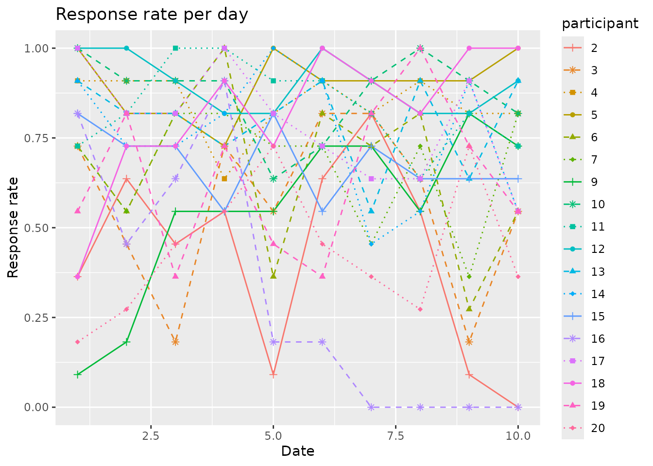
We also suggest a way to plot the participant response rates, to
identify patterns like response rates dropping over time. For this, we
provide the plot_response_rate() function.
plot_response_rate(
  data = example_data,
  time_col = sent,
  participant_col = participant,
  valid_col = answered
)
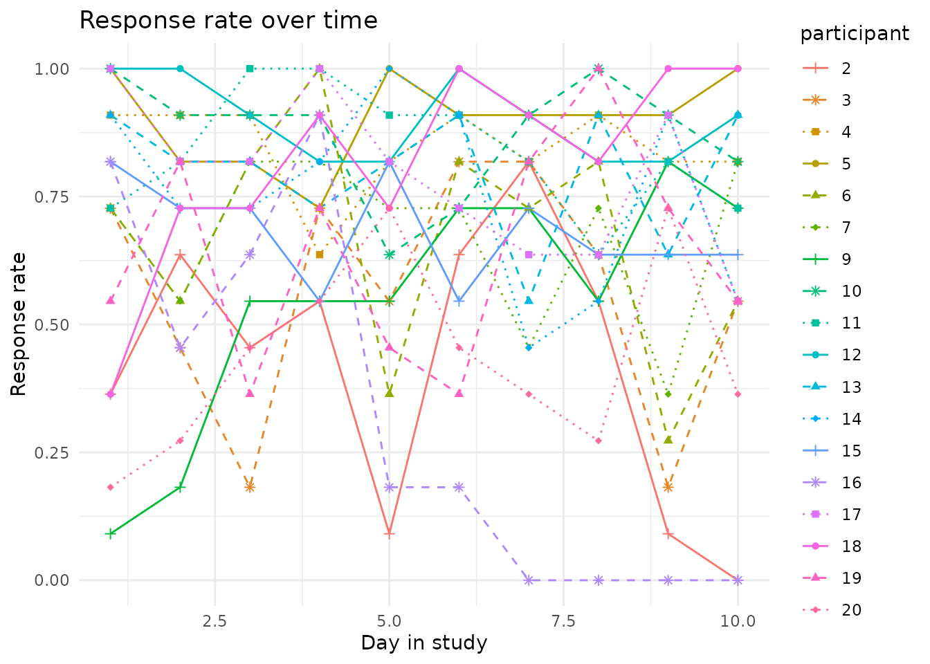
Note that the resulting plot can be further customized using the
ggplot2 package.
library(ggplot2)

plot_response_rate(
  data = example_data,
  time_col = sent,
  participant_col = participant,
  valid_col = answered
) +
  theme_minimal() +
  ggtitle('Response rate over time') +
  xlab('Day in study')
